Real Time Wave Prediction Using Neural Networks at Karwar, West Coast of India-Juniper Publishers
Juniper Publishers- Journal of Oceanography
Abstract
The knowledge of ocean waves is an essential prerequisite for almost all activities in ocean. Traditional methods have disadvantages of excessive data requirement, time consumption and are tedious to carry out. ANN is being widely applied in coastal engineering field since last two decades in variety of time series forecasting. Study has been carried out to predict waves using FFBP and NARX networks. Wave data obtained from INCOIS is made use in the present study. Effect of network architecture on the performance of the model has been studied. It was found that for time series prediction NARX network outperforms FFBP.
Keywords: Artificial neural network; Feed forward back propagation network; Non-linear auto regressive with exogenous input; Coastal engineering
Introduction
Accurate forecasting of wave characteristics is important for many coastal and marine activities. Different methods have been developed for this purpose. There are many empirical formulae for wave growth which have been derived from large visually observed data sets. The curves developed by Sverdrup and Munk in 1947 and Pierson, Neumann and James in 1955 (PNJ) were also used for wave forecasting. These two number of visual observations by graphical methods using known parameters of wave characteristics. Its major disadvantage is the time necessary to make the computations and also it requiring large information about oceanographic and meteorological data.
A new model based on the working of human brain has been idealized to meet the objective of learning relationship between complex parameters involved in the interaction without having to know the underlying physics behind it. As it is an attempt to mimic the capabilities of human neural system it is called Artificial Neural Network (ANN). An extensive literature survey has been carried out to understand the dynamics of ocean waves, their interactions and transformations. As the subject is very vast only some relevant literature which implemented the neural network for wave forecasting has been presented. [1] describes the application of neural network analysis in forecasting of significant wave height with 3 hour lead period. Wave forecasting was done using wind velocity, fetch and duration as input parameters by [2]. The results were not satisfactory fetch and duration was excluded as their presence did not have any effect on predictions. After MuCulloch and introduced the concept of ANN, many models were developed. Among those models the multi-layered network trained by back propagation algorithm has been applied extensively to solve various engineering problems by [3]. They reported an application of the feed forward neural network to forecast the wave heights of a site based on the observed wave data of other sites at Taichung Harbor. Results showed that wave forecast of a local site has a better performance when the wave data of multisite observations are used. The most common training algorithm is the standard back-propagation (BP), although numerous training schemes are available to impart better training with the same set of data as shown by [4] in their harbor tranquility studies. The work carried out by [5] describes hind casting of wave heights and periods from cyclone generated wind fields using two input configurations of neural network. They use updated algorithms in back propagation neural network and the wave forecasting yielded better results. Deo MC [6] describes the application of neural network analysis in forecasting of significant wave height with 3 hour lead period. They have carried out different combinations of training patterns to obtain the desired output in addition to the work of average 12 hour and a day wave forecasting. They used three different algorithms of back propagation, conjugate gradient descent and cascade correlation to predict wave height. Tsai CP [3] used back propagation neural network to forecast the ocean waves based on learning characteristics of observed waves and also based on wave records at the neighboring stations. Dwarakish GS [4] carried out a study to predict the breaking wave height and depth using five different datasets. Deo M [7] explained multilayered feed forward and recurrent networks with conjugate gradient and steepest descent with momentum method to predict waves and compared the results with those obtained from stochastic models of Auto Regressive and Auto Regressive eXogenous input models. Sensitivity analysis showed that wind speed and direction is the most important parameter for wave hind casting. Present study utilizes the advantages of Feed Forward Back Propagation (FFBP) and Non-linear Auto Regressive eXogenous (NARX) networks for prediction of waves [8-10].
Methods
FFBP network
Development of ANN can be attributed to the attempt carried out to mimic the working pattern of human brain. Its success lies in its ability to exploit the non-linear relationship between input and output data by continuously adapting itself to the information provided to it by means of some learning process. ANN can be classified based on network type in to feed forward and feedback or recurrent networks. The basic difference between the two is that, in feed forward networks the information is passed from one layer to the other in a forward manner till the output is obtained in the output layer. Whereas in, feedback network the output obtained in the output layer is fed back in to the network through input layer thus this type of network will have minimum of single loop in its structure. A neural network consisting of a set of connected cells called the neurons. A graphical representation of neuron is given in Figure 1.
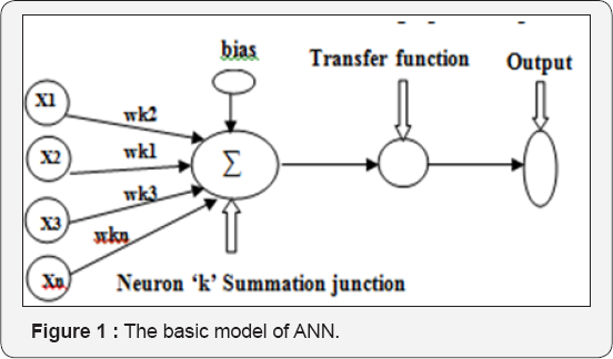
A neuron is a real function of input vectors xl, x2, x3....xn and wkl, wk2, wk3...wkn are the weights associated with the connections i.e. synaptic weight connections from input neuron 'i' to neuron 'k'. 'k' neuron is the summing junction where net input is given by
uk = Σ wki* xi (1)
vk=uk+bk (2)
bk is the bias value at the kth neuron.
The output yk is the transformed weighted sum of vk
Yk = ⌉ (vk) (3)
Where,  is the transfer function or activation function used to convert the summed input. A nonlinear sigmoid function which is monotonically increasing and continuously differentiable is the most commonly used activation function. It can be mathematically expressed as,
Yk = ⌉(vk) = 1/(1+exp(-avk))
Once the activities of all output units have been determined, the network computes the error E, which is defined by the expression.
E = 1/2Σ(yi - di) 2 (5)

Where yi is the activity level of the ith unit in the top layer and di is the desired output of the ith unit. The most commonly used learning algorithm in coastal engineering application is the gradient descent algorithm. In this the global error calculated is propagated backward to the input layer through weight connections as in Figure 2, during which the weights are updated in the direction of steepest descent or in the direction opposite to gradient descent. However the overall objective of any learning algorithm is to reduce the global error, E defined as
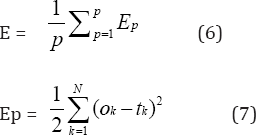
Where Ep is the error at the pth training pattern, Ok is the obtained output from network at the kth output node and tk is the target output kth output node and N is the total number of output nodes. Levenberg-Marquardt algorithm used in this study can be written as
Wnew=Wold-[JT+γl]-1JTE(Wold) (8)
Where J is the Jacobian matrix that contains first derivatives of the network errors with respect to the weights and biases, I is the identity matrix and γ is the parameter used to define the iteration step value. It minimizes the error function while trying to keep the step between old weight configuration (Wold) and new updated one (Wnew). The performance of the network is measured in terms of various performance functions like mean squared error (MSE or 'mse'), root mean squared error (RMSE) and Co-efficient of Correlation (CC or 'R') between the predicted and the observed values of the quantities [11-13].
NARX network
In the present study along with FFBP, a recurrent type of network namely Non-linear Auto Regressive network with exogenous inputs (NARX) has also been used. In recurrent networks, the output depends not only on the current input to the network but also on the previous input and output of the network. The response of the static network at any point of time depends only on the value of the input sequence at that same point whereas, the response of the recurrent networks lasts longer than the input pulse. This is done by introducing a tapped delay line in the network which makes the input pulse last longer than its duration by an amount which is equal to the delay given in the tapped delay. This makes network to have a memory of the input that is fed. The defining equation for the NARX model is
y(t) = f( y(t-1), y(t-2),.... y(t-ny), u(t-1), u(t-2) u(t-nu)) (9)

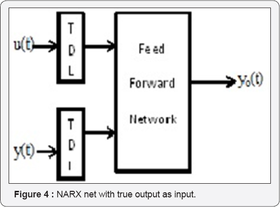
Where, the next value of the dependent output signal y(t) is regressed on previous values of an independent (exogenous) input signal. The output of NARX network can be considered to be an estimate of the output of some non-linear dynamic system that is being modeled. The output is fed back to the input of the feed forward network in standard NARX architecture as shown in Figure 3. Since the true output is available during training, the true output itself can be used instead of feeding back the estimated output as shown in Figure 4. This will have two advantages. The first is that the input to the feed forward network is more accurate. The second is that the resulting network has a purely FFBP architecture and static back propagation can be used for training instead of dynamic back propagation, which has complex error surfaces exposing the network to higher chances of getting trapped in local minima and hence requiring more number of training iterations [14-16].
Network parameters and performance indicators
Three layered FFBP network with single input layer, hidden layer and output layer was used. Tangent sigmoid (tansig) was used in the hidden layer as transfer function as data was normalized to fall in the range of -1 to 1 and purely linear (purelin) transfer function was used in the output layer, as this combination of 'tansig' and 'purelin' transfer function is capable of approximating any function. The training was carried out using the aforementioned network architecture for various data size matrices. The number of the neurons in the hidden layer was kept on increasing starting from one, till the best combination was found in terms of network performance indicators. One thousand iterations were set as the stopping criteria for the training of the network. The performance of the network is measured in terms of various performance indicators like sum squared error (SSE), mean squared error (MSE), root mean squared error (RMSE) and co-efficient of correlation (CC or 'R') between the predicted and the observed values of the quantities. In the present study 'mse' and 'R' are used as performance indicators; lower value of MSE and higher value of 'R' indicates better performance of the network.
Mean square error: In statistics, the mean squared error of an estimator measures the average of the squares of the 'errors', ie., the difference between the estimator and what is estimated. It is given by the formula
mse = Σ(xi-yi)2/n (10)
Correlation co-efficient: It measures the strength of association between the variables also it represents the direction of the linear relationship between two variables that is defined as the covariance divided by the product of their standard deviations and is given by the formula:
R = Σ(Xi.yi)/√(Σxi2).(Σyi2) (11)
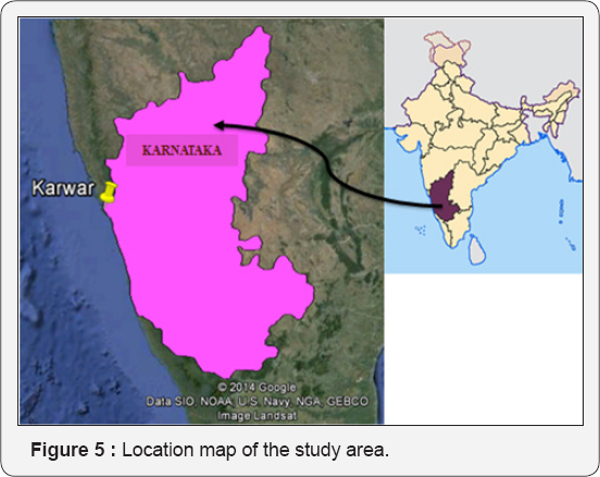
Study area and data division: The study is carried out for Off Karwar coast located at northern tip in the coastal segment of Karnataka state, along west coast of India. It lies between 14.083 North latitude and 74.083 East longitude as shown in Figure 5.
FFBP and NARX networks have been used for the prediction of waves at Karwar. Significant wave height from January 2011 to December 2013 obtained from Indian National Centre for Ocean Information Services (INCOIS) is made use of in the present study. Predictions were carried out for various length of duration using a week's data and month's data as input. The data was divided into weekly and monthly data sets for the prediction of waves using various duration of data sets. In weekly data sets a row in a input matrix comprises of 336 data points. These rows represent a single node in the input and output layer of the network. Similarly in monthly data sets a single row consists of 1440 data points. In the present study yearly data sets were divided into 12 months consisting of 30 days each for the regularity of input data matrix size.
Results and Discussion
Prediction with FFBP network
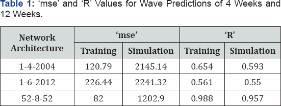
In the present study four week’s prediction was carried out using one week's wave data from 01/01/2011 to 07/01/2011 as input. The target data set comprised readings of four weeks duration from 08/01/2011 to 04/02/2011 (28 days), a week’s data having 336 time steps represent a single node in this case, similarly output layer consists of four nodes for four weeks of data. Subsequent weeks in similar fashion were given as input and target for testing the trained network. The ‘R’ values showed marginal increase in 4 weeks prediction which might be due to the increased number of target values available for the network generalization. However the ‘R’ value decreased for the 12 weeks significant wave height as one week's input data range was too small for predicting a long duration of 12 weeks wave height. The number of neurons was increased in hidden layer by one after every prediction. The best performance was obtained at four and six neurons in hidden layer during 4 weeks and 12 weeks prediction of significant wave height. The training performance showed considerable increase in 'R' values but testing 'R' values drastically reduced hinting at the overfitting behaviour of the network when the number of neurons was increased beyond four and six during 4 weeks and 12 weeks significant wave height prediction when number of neurons in hidden layer was increased. In both the cases the prediction duration is large (4 weeks and 12 weeks) compared to input data of one week. Table 1 gives the results of weekly prediction duration of four weeks and twelve weeks using one week’s data as input. Naturally the range of targets will be greater than those of input provided, weakening the prediction capability of the network when new data set is fed to the network.
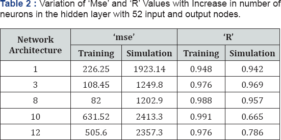

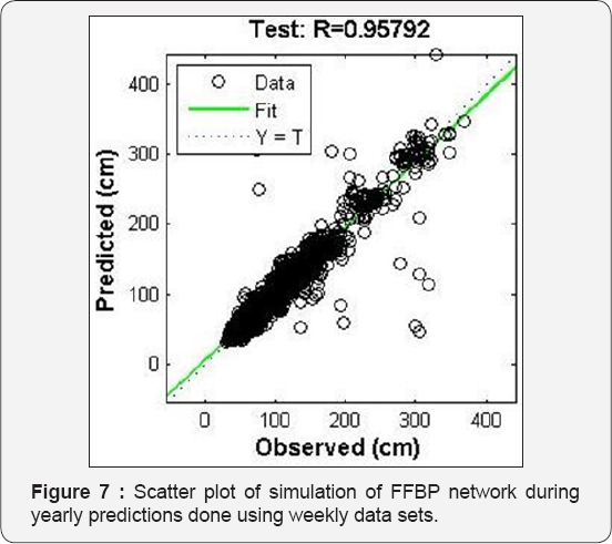
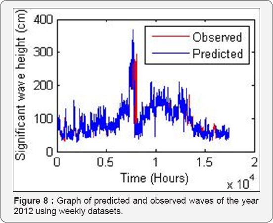
Similarly, yearlong predictions are carried out using data of year 2011 as input and data of year 2012 as target in training process and next two consecutive year’s data (2012 and 2013) as input and target for simulation purpose respectively. The input and output layer consist of 52 nodes representing 52 weeks data for a single year. The prediction done using yearlong data yielded satisfactory results with training process 'R' value reaching up to 0.988 and simulation 'R' value reaching up to 0.957. The optimum number of neurons beyond eight led to decrease in the prediction capability of the trained network when simulation data sets are presented to the network as seen in Table 2. The scatter plot of training and simulation of the network is shown in Figure 6 & 7. The plot of observed values and predicted values is shown in the Figure 8.
Monthly prediction involved feeding the network with a month’s data having 1440 data points in a single input node. The year 2011 hourly wave data were divided into twelve sets having 1440 data points each corresponding to 30 days of observation, hence the yearly data comprised of 01/01/2011 to 26/12/2011 (360 days). For one month’s wave prediction data from 01/01/2011 to 30/01/2011 and from 31/01/2011 to 01/03/2011 was given as input and target data respectively. The subsequent data of 30 days period were given as input and targets for testing purpose. The number of neurons was increased in the hidden layers, however not much appreciable improvement was seen hence the number of neurons was taken as one for all the forthcoming predictions which has a month's data as input in a single node which involved one month's data as input as shown in Table 3.
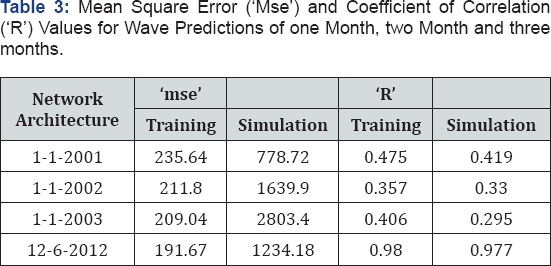
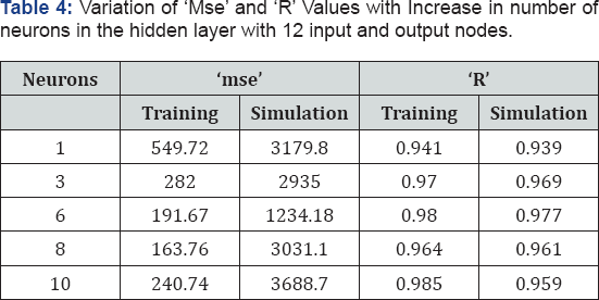
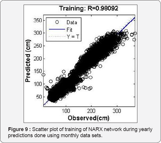
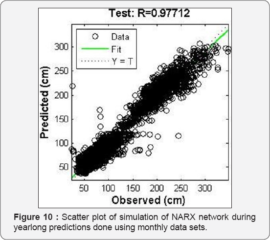
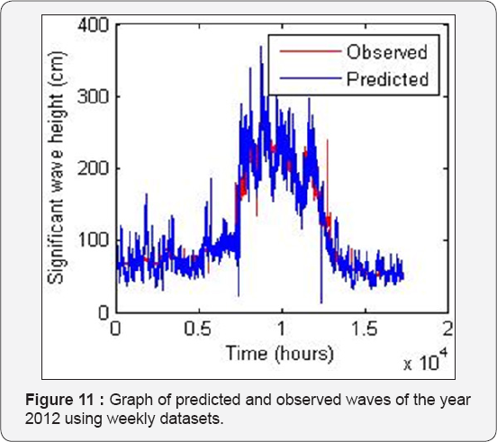
A year’s data set contains 17592 readings however this was cut short to 17472 readings so that the data can be divided equally in to 12 months comprising of 30 days (1440 readings) each. Prediction for entire year using 12 months data of year 2011 as input with equal number of input nodes is carried out giving the year 2012 wave data of 12 months as target during the training process. The trained network is then used to predict the 2012 wave data using 2011 wave data as input. The results obtained are very good in this case and 'mse' value as low as 191.67 and 1234.18 were obtained for training and simulation respectively, also high 'R' value of 0.980 and 0.977 were obtained. The optimum number of neuron in hidden layer is found to be six in this case. The increase in number of neurons beyond six led to decrease in the prediction capability of the trained network when simulation data sets are presented to the network as seen in Table 4. Figure 9 & 10 gives the scatter plot of training and simulation of the network. The plot of observed values and predicted values are shown in the Figure 11.
Prediction with NARX network
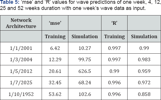
Data was divided into weekly and monthly sets in a similar fashion as done for the purpose of prediction of waves using FFBP network. Weekly predictions were carried out using one week’s data to predict 4, 12, 25 and 52 weeks wave predictions respectively. The results obtained in terms of 'mse' and 'R' was good ranging from 0.99 for one week's prediction to greater than 0.97 for 25 weeks prediction. However the accuracy dropped to 0.85 for predictions of 52 week wave data using one week's data. The use of target data as one of the input nodes as explained in Figure 3 helped in improving the efficiency of the network and also in long term prediction of wave data using small amount of data. The best performance for prediction of 25 weeks was obtained for seven numbers of neuron in the hidden layer. The variation of 'R' values for the case is shown in Table 5.
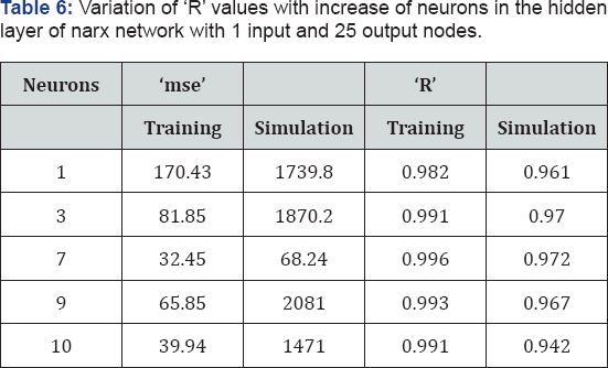

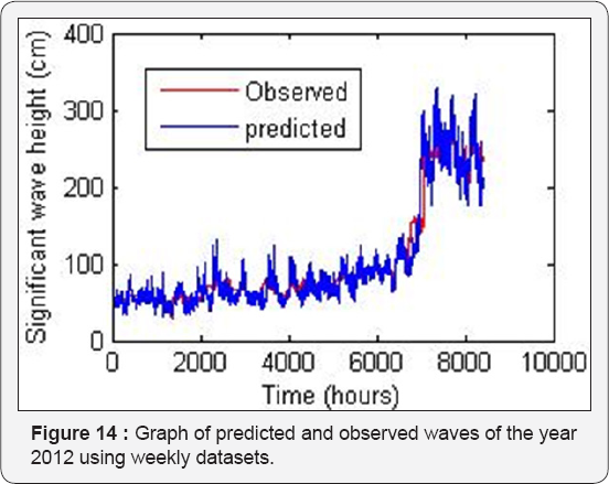
The increase in number of neurons beyond seven led to decrease in the prediction capability of the trained network when simulation data sets are presented to the network as seen in Table 6. Scatter plot and graph observed versus predicted waves are shown in Figure 12-14.
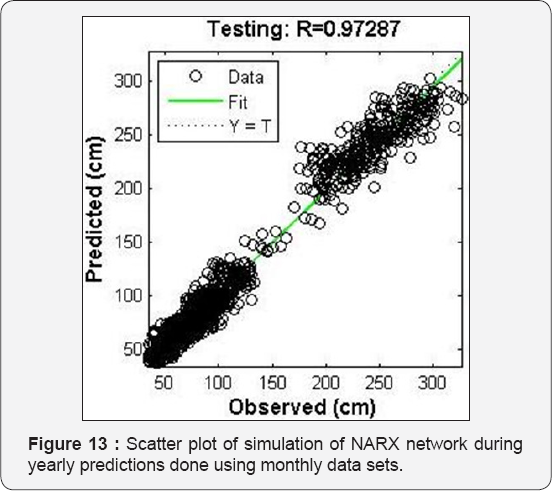
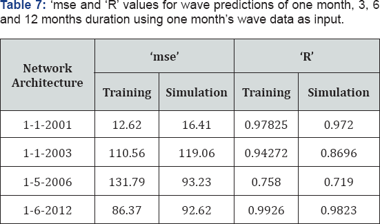
Monthly predictions were also carried out on similar lines using one month data set for predictions of wave height with duration ranging from one month to twelve months the results of which are tabulated in the Table 7. January 2011's data used as input and subsequent months as target for all training iterations of various lengths of predictions. One year's prediction can be obtained with accuracy greater than 0.98. Also the NARX network's results in both the weekly and monthly analysis showed steady decrease in accuracy when the duration of prediction was increased keeping the input data length as constant. The increase in neurons in the hidden layer beyond the best network architecture also showed gradual decrease in accuracy rather than varied ones which would have rendered the study inconclusive.
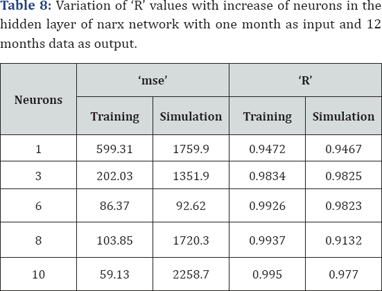
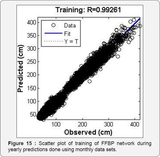
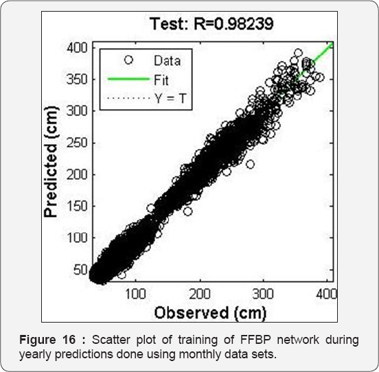
The increase in number of neurons beyond six led to decrease in the prediction capability of the trained network when simulation data sets are presented to the network as seen in Table 8. Scatter plot of training and simulation are shown in Figure 15 & 16. The graph of observed and predicted values are shown in Figure 17.

Conclusion
Traditional methods of predictions of waves were carried based on semi empirical formulations and numerical modeling which is data intensive. The present study makes use of relatively new technique of ANN which has been tried and tested in various coastal engineering applications. Predictions for yearlong significant wave height using equal length of input data of weekly and monthly sets gave satisfactory results in FFBP network with co-efficient of correlation values greater than 0.95 in both the cases. Whereas, using the NARX network, one week's data was successfully utilized to predict waves at the same location for six months duration with 'R' value greater than 0.86. The yearlong prediction using one month’s data gave good 'R' value of 0.97. The NARX network outperformed FFBP network in terms of data requirement and accuracy achieved also it takes less computational time as well.
Comments
Post a Comment